42 how to put data labels in excel chart

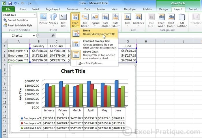
Excel charts: add title, customize chart axis, legend and data labels Click anywhere within your Excel chart, then click the Chart Elements button and check the Axis Titles box. If you want to display the title only for one axis, either horizontal or vertical, click the arrow next to Axis Titles and clear one of the boxes: Click the axis title box on the chart, and type the text. How to Create a Bar Chart With Labels Above Bars in Excel In the chart, right-click the Series "# Footballers" Data Labels and then, on the short-cut menu, click Format Data Labels. 9. In the Format Data Labels pane, under Label Options selected, set the Label Position to Inside Base. 10. Then, under Label Contains, check the Category Name option and uncheck the Value and Show Leader Lines options. 11.

How to Insert Axis Labels In An Excel Chart | Excelchat We will again click on the chart to turn on the Chart Design tab We will go to Chart Design and select Add Chart Element Figure 6 - Insert axis labels in Excel In the drop-down menu, we will click on Axis Titles, and subsequently, select Primary vertical Figure 7 - Edit vertical axis labels in Excel

How to put data labels in excel chart

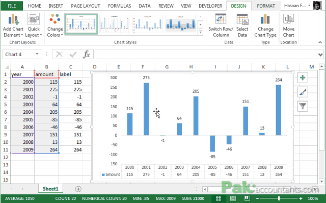
Add or remove data labels in a chart - Microsoft Support Click the data series or chart. To label one data point, after clicking the series, click that data point. In the upper right corner, next to the chart, click Add Chart Element > Data Labels. To change the location, click the arrow, and choose an option. If you want to show your data label inside a text bubble shape, click Data Callout. Add a DATA LABEL to ONE POINT on a chart in Excel Steps shown in the video above: Click on the chart line to add the data point to. All the data points will be highlighted. Click again on the single point that you want to add a data label to. Right-click and select ' Add data label ' This is the key step! Right-click again on the data point itself (not the label) and select ' Format data label '. Chart elements excel - klki.ekstrabut.pl Follow the steps given below to insert the chart elements in your graph. Step 1 − Click the chart . Three buttons appear at the upper-right corner of the chart . They are − Chart Elements Chart Styles and Colors, and Chart Filters Step 2 − Click the Chart Elements icon. A list of available elements will be displayed.

How to put data labels in excel chart. Adding rich data labels to charts in Excel 2013 | Microsoft 365 Blog Putting a data label into a shape can add another type of visual emphasis. To add a data label in a shape, select the data point of interest, then right-click it to pull up the context menu. Click Add Data Label, then click Add Data Callout . The result is that your data label will appear in a graphical callout. Add data labels to your Excel bubble charts | TechRepublic Right-click the data series and select Add Data Labels. Right-click one of the labels and select Format Data Labels. Select Y Value and Center. Move any labels that overlap. Select the data labels ... How To Use Dynamic Data Labels To Create Interactive Excel Charts To create a column chart with dynamic data labels, you need to follow these given steps. Select the data & Create a Combo Chart. Now select the column chart for revenue data and a line chart with marker for data labels. Add Data Labels to the Line Chart With Marker. After then remove the Line Color and Marker Color. How to Add Labels to Scatterplot Points in Excel - Statology Step 3: Add Labels to Points. Next, click anywhere on the chart until a green plus (+) sign appears in the top right corner. Then click Data Labels, then click More Options…. In the Format Data Labels window that appears on the right of the screen, uncheck the box next to Y Value and check the box next to Value From Cells.

how to add data labels into Excel graphs - storytelling with data You can download the corresponding Excel file to follow along with these steps: Right-click on a point and choose Add Data Label. You can choose any point to add a label—I'm strategically choosing the endpoint because that's where a label would best align with my design. Excel defaults to labeling the numeric value, as shown below. How to Add Data Labels to an Excel 2010 Chart - dummies On the Chart Tools Layout tab, click Data Labels→More Data Label Options. The Format Data Labels dialog box appears. You can use the options on the Label Options, Number, Fill, Border Color, Border Styles, Shadow, Glow and Soft Edges, 3-D Format, and Alignment tabs to customize the appearance and position of the data labels. How to add data labels from different column in an Excel chart? Right click the data series in the chart, and select Add Data Labels > Add Data Labels from the context menu to add data labels. 2. Click any data label to select all data labels, and then click the specified data label to select it only in the chart. 3. Add / Move Data Labels in Charts - Excel & Google Sheets Adding Data Labels Click on the graph Select + Sign in the top right of the graph Check Data Labels Change Position of Data Labels Click on the arrow next to Data Labels to change the position of where the labels are in relation to the bar chart Final Graph with Data Labels

Add data labels and callouts to charts in Excel 365 | EasyTweaks.com Step #1: After generating the chart in Excel, right-click anywhere within the chart and select Add labels . Note that you can also select the very handy option of Adding data Callouts. How to Change Excel Chart Data Labels to Custom Values? First add data labels to the chart (Layout Ribbon > Data Labels) Define the new data label values in a bunch of cells, like this: Now, click on any data label. This will select "all" data labels. Now click once again. At this point excel will select only one data label. Go to Formula bar, press = and point to the cell where the data label ... How to Use Cell Values for Excel Chart Labels Select the chart, choose the "Chart Elements" option, click the "Data Labels" arrow, and then "More Options." Uncheck the "Value" box and check the "Value From Cells" box. Select cells C2:C6 to use for the data label range and then click the "OK" button. The values from these cells are now used for the chart data labels. How to Place Labels Directly Through Your Line Graph in Microsoft Excel Right-click on top of one of those circular data points. You'll see a pop-up window. Click on Add Data Labels. Your unformatted labels will appear to the right of each data point: Click just once on any of those data labels. You'll see little squares around each data point. Then, right-click on any of those data labels. You'll see a pop-up menu.

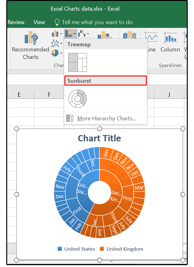
What to do with Excel 2016's new chart styles: Treemap, Sunburst, and Box & Whisker | PCWorld

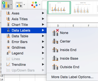
Adding Data Labels to Your Chart (Microsoft Excel) To add data labels in Excel 2013 or Excel 2016, follow these steps: Activate the chart by clicking on it, if necessary. Make sure the Design tab of the ribbon is displayed. (This will appear when the chart is selected.) Click the Add Chart Element drop-down list. Select the Data Labels tool.

Add labels to a Google chart or graph - YouTube

How to create Custom Data Labels in Excel Charts Two ways to do it. Click on the Plus sign next to the chart and choose the Data Labels option. We do NOT want the data to be shown. To customize it, click on the arrow next to Data Labels and choose More Options … Unselect the Value option and select the Value from Cells option. Choose the third column (without the heading) as the range.

How to Make Charts and Graphs in Excel | Smartsheet

Custom Chart Data Labels In Excel With Formulas Follow the steps below to create the custom data labels. Select the chart label you want to change. In the formula-bar hit = (equals), select the cell reference containing your chart label's data. In this case, the first label is in cell E2. Finally, repeat for all your chart laebls.

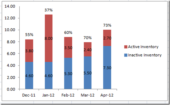
How-to Put Percentage Labels on Top of a Stacked Column Chart - Excel Dashboard Templates

How to Add Data Labels in Excel - Excelchat | Excelchat After inserting a chart in Excel 2010 and earlier versions we need to do the followings to add data labels to the chart; Click inside the chart area to display the Chart Tools. Figure 2. Chart Tools Click on Layout tab of the Chart Tools. In Labels group, click on Data Labels and select the position to add labels to the chart. Figure 3.

Data labels on Excel charts « projectwoman.com

Edit titles or data labels in a chart - support.microsoft.com On a chart, click one time or two times on the data label that you want to link to a corresponding worksheet cell. The first click selects the data labels for the whole data series, and the second click selects the individual data label. Right-click the data label, and then click Format Data Label or Format Data Labels.

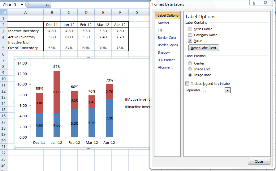
Excel Dashboard Templates How-to Put Percentage Labels on Top of a Stacked Column Chart - Excel ...

How to use data labels in a chart - YouTube Excel charts have a flexible system to display values called "data labels". Data labels are a classic example a "simple" Excel feature with a huge range of o...

How to Add Data Labels to your Excel Chart in Excel 2013 - YouTube

Excel tutorial: How to use data labels Generally, the easiest way to show data labels to use the chart elements menu. When you check the box, you'll see data labels appear in the chart. If you have more than one data series, you can select a series first, then turn on data labels for that series only. You can even select a single bar, and show just one data label.

Excel Dashboard Templates How-to Use Data Labels from a Range in an Excel Chart - Excel ...

How to add or move data labels in Excel chart? - ExtendOffice In Excel 2013 or 2016. 1. Click the chart to show the Chart Elements button . 2. Then click the Chart Elements, and check Data Labels, then you can click the arrow to choose an option about the data labels in the sub menu. See screenshot: In Excel 2010 or 2007. 1. click on the chart to show the Layout tab in the Chart Tools group. See ...

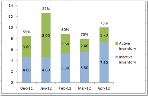
How-to Put Percentage Labels on Top of a Stacked Column Chart - Excel Dashboard Templates

How to Add Total Data Labels to the Excel Stacked Bar Chart Step 4: Right click your new line chart and select "Add Data Labels" Step 5: Right click your new data labels and format them so that their label position is "Above"; also make the labels bold and increase the font size. Step 6: Right click the line, select "Format Data Series"; in the Line Color menu, select "No line"

How to Add Data Labels to an Excel 2010 Chart - dummies

How to Create a Bar Chart With Labels Inside Bars in Excel In the chart, right-click the Series "# Footballers" Data Labels and then, on the short-cut menu, click Format Data Labels. 8. In the Format Data Labels pane, under Label Options selected, set the Label Position to Inside End. 9. Next, in the chart, select the Series 2 Data Labels and then set the Label Position to Inside Base. 10.

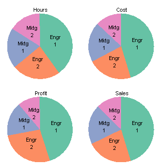
Column Chart to Replace Multiple Pie Charts - Peltier Tech Blog

Chart elements excel - klki.ekstrabut.pl Follow the steps given below to insert the chart elements in your graph. Step 1 − Click the chart . Three buttons appear at the upper-right corner of the chart . They are − Chart Elements Chart Styles and Colors, and Chart Filters Step 2 − Click the Chart Elements icon. A list of available elements will be displayed.

Excel rotate radar chart - Stack Overflow

Add a DATA LABEL to ONE POINT on a chart in Excel Steps shown in the video above: Click on the chart line to add the data point to. All the data points will be highlighted. Click again on the single point that you want to add a data label to. Right-click and select ' Add data label ' This is the key step! Right-click again on the data point itself (not the label) and select ' Format data label '.