38 scatter chart in excel with labels
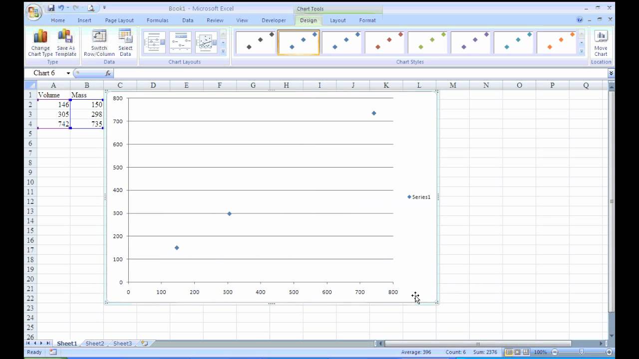
How To Create Scatter Chart in Excel? - EDUCBA To apply the scatter chart by using the above figure, follow the below-mentioned steps as follows. Step 1 - First, select the X and Y columns as shown below. Step 2 - Go to the Insert menu and select the Scatter Chart. Step 3 - Click on the down arrow so that we will get the list of scatter chart list which is shown below. Scatter Graph - Overlapping Data Labels - Excel Help Forum Unfortunately the attachment icon doesn't work at the moment, so to attach an Excel file you have to do the following: just before posting, scroll down to Go Advanced and then scroll down to Manage Attachments. Now follow the instructions at the top of that screen.
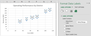
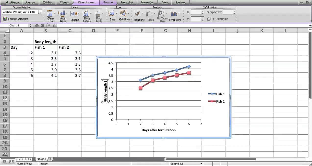
How to Add Labels to Scatterplot Points in Excel - - Statology Step 3: Add Labels to Points. Next, click anywhere on the chart until a green plus (+) sign appears in the top right corner. Then click Data Labels, then click More Options…. In the Format Data Labels window that appears on the right of the screen, uncheck the box next to Y Value and check the box next to Value From Cells.
Scatter chart in excel with labels
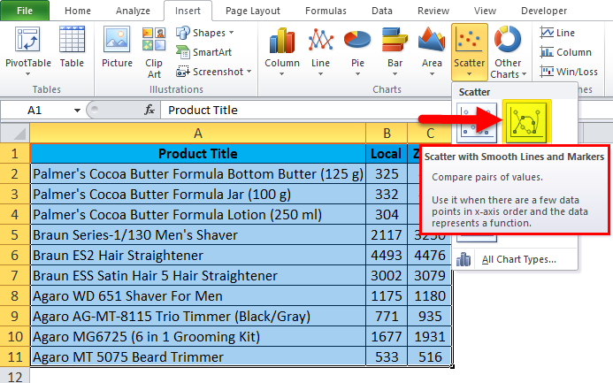
Scatter Plot with Text Labels on X-axis : excel LET is excellent for dealing with complex formulas that reuse the same "variable" multiple times. For example, consider a formula like this: =IF (XLOOKUP (A1,B:B,C:C)>5,XLOOKUP (A1,B:B,C:C)+3,XLOOKUP (A1,B:B,C:C)-2) So basically a lookup or something else with a bit of complexity, is referenced multiple times. Add Custom Labels to xy Scatter plot in Excel Step 1: Select the Data, INSERT -> Recommended Charts -> Scatter chart (3 rd chart will be scatter chart) Let the plotted scatter chart be. Step 2: Click the + symbol and add data labels by clicking it as shown below. Step 3: Now we need to add the flavor names to the label. Now right click on the label and click format data labels. How to display text labels in the X-axis of scatter chart in Excel? Display text labels in X-axis of scatter chart Actually, there is no way that can display text labels in the X-axis of scatter chart in Excel, but we can create a line chart and make it look like a scatter chart. 1. Select the data you use, and click Insert > Insert Line & Area Chart > Line with Markers to select a line chart. See screenshot: 2.
Scatter chart in excel with labels. Add or remove data labels in a chart - support.microsoft.com Click the data series or chart. To label one data point, after clicking the series, click that data point. In the upper right corner, next to the chart, click Add Chart Element > Data Labels. To change the location, click the arrow, and choose an option. If you want to show your data label inside a text bubble shape, click Data Callout. How to display text labels in the X-axis of scatter chart in ... Display text labels in X-axis of scatter chart. Actually, there is no way that can display text labels in the X-axis of scatter chart in Excel, but we can create a line chart and make it look like a scatter chart. 1. Select the data you use, and click Insert > Insert Line & Area Chart > Line with Markers to select a line chart. See screenshot: Excel: labels on a scatter chart, read from array - Stack Overflow Excel: labels on a scatter chart, read from array Ask Question 0 Here I have a chart I did a right-click -> "Add labels" , and it read them from my a (H/C) row. Basically, I want it to read label values from the CO2/CH4 row instead, so they would be 0,0.5,1,2,5,10 instead. How to add text labels on Excel scatter chart axis - Data Cornering Add dummy series to the scatter plot and add data labels. 4. Select recently added labels and press Ctrl + 1 to edit them. Add custom data labels from the column "X axis labels". Use "Values from Cells" like in this other post and remove values related to the actual dummy series. Change the label position below data points.
Use text as horizontal labels in Excel scatter plot Edit each data label individually, type a = character and click the cell that has the corresponding text. This process can be automated with the free XY Chart Labeler add-in. Excel 2013 and newer has the option to include "Value from cells" in the data label dialog. Format the data labels to your preferences and hide the original x axis labels. How to Find, Highlight, and Label a Data Point in Excel Scatter Plot? By default, the data labels are the y-coordinates. Step 3: Right-click on any of the data labels. A drop-down appears. Click on the Format Data Labels… option. Step 4: Format Data Labels dialogue box appears. Under the Label Options, check the box Value from Cells . Step 5: Data Label Range dialogue-box appears. Excel Chart Vertical Axis Text Labels - My Online Training Hub Apr 14, 2015 · So all we need to do is get that bar chart into our line chart, align the labels to the line chart and then hide the bars. We’ll do this with a dummy series: Copy cells G4:H10 (note row 5 is intentionally blank) > CTRL+C to copy the cells > select the chart > CTRL+V to paste the dummy data into the chart. How to create a scatter plot and customize data labels in Excel During Consulting Projects you will want to use a scatter plot to show potential options. Customizing data labels is not easy so today I will show you how th...
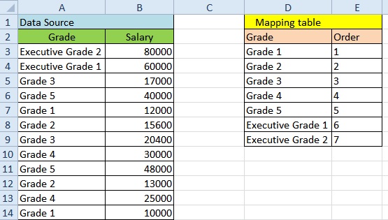
Scatter Plots in Excel with Data Labels Select "Chart Design" from the ribbon then "Add Chart Element" Then "Data Labels". We then need to Select again and choose "More Data Label Options" i.e. the last option in the menu. This will... Excel scatter chart using text name - Access-Excel.Tips Solution - Excel scatter chart using text name To group Grade text (ordinal data), prepare two tables: 1) Data source table 2) a mapping table indicating the desired order in X-axis In Data Source table, vlookup up "Order" from "Mapping Table", we are going to use this Order value as x-axis value instead of using Grade. How do I set labels for each point of a scatter chart? Click one of the data points on the chart. Chart Tools. Layout contextual tab. Labels group. Click on the drop down arrow to the right of:- Data Labels Make your choice. If my comments have helped please vote as helpful. Thanks. Report abuse Was this reply helpful? Yes No How to Make a Scatter Plot in Excel (XY Chart) Data Labels — Do add the data labels to the scatter chart, select the chart, click on the plus icon on the right, and then check the data labels option.
Scatter Plot with multiple series and filtering/sorting on values other than the series name : excel
How to label scatterplot points by name? - Stack Overflow 13 Apr 2016 — right click on your data point · select "Format Data Labels" (note you may have to add data labels first) · put a check mark in "Values from Cells ...
Scatter Chart in Excel (Examples) | How To Create Scatter Chart in Excel?
How to use a macro to add labels to data points in an xy ... The labels and values must be laid out in exactly the format described in this article. (The upper-left cell does not have to be cell A1.) To attach text labels to data points in an xy (scatter) chart, follow these steps: On the worksheet that contains the sample data, select the cell range B1:C6.
Creating a scatter chart in Excel for iPad? - Microsoft Community
How to find, highlight and label a data point in Excel scatter plot To let your users know which exactly data point is highlighted in your scatter chart, you can add a label to it. Here's how: Click on the highlighted data point to select it. Click the Chart Elements button. Select the Data Labels box and choose where to position the label.

Add Custom Labels to x-y Scatter plot in Excel - DataScience Made Simple
How to Change Excel Chart Data Labels to Custom Values? May 05, 2010 · The Chart I have created (type thin line with tick markers) WILL NOT display x axis labels associated with more than 150 rows of data. (Noting 150/4=~ 38 labels initially chart ok, out of 1050/4=~ 263 total months labels in column A.) It does chart all 1050 rows of data values in Y at all times.
Scatter Chart in Excel (Examples) | How To Create Scatter Chart in Excel?
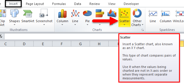
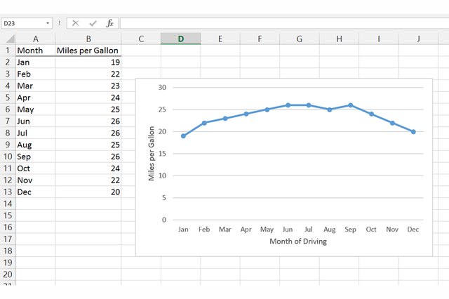
how to make a scatter plot in Excel - storytelling with data Select "Scatter" from the options in the "Recommended Charts" section of your ribbon. Excel will automatically create a scatter plot for you in the same sheet as your data, using the first column of your dataset as the horizontal (X) axis, and the second column as your vertical (Y) axis. A quick note here: in creating scatter plots, a ...
3d scatter plot for MS Excel
How to create a scatter plot in Excel - Ablebits.com 29 Mar 2022 — Add labels to scatter plot data points · Select the plot and click the Chart Elements button. · Tick off the Data Labels box, click the little ...

Scatter Chart in Microsoft Excel
Excel scatter plot with legend Display text labels in X-axis of scatter chart. Actually, there is no way that can display text labels in the X-axis of scatter chart in Excel, but we can create a line chart and make it look like a scatter chart. 1. Select the data you use, and click Insert > Insert Line & Area Chart > Line with Markers to select a line chart.
Excel Charts | Real Statistics Using Excel
Present your data in a scatter chart or a line chart Scatter charts and line charts look very similar, especially when a scatter chart is displayed with connecting lines. However, the way each of these chart types plots data along the horizontal axis (also known as the x-axis) and the vertical axis (also known as the y-axis) is very different.

Improve your X Y Scatter Chart with custom data labels
Scatter Plot Chart in Excel (Examples) | How To Create Scatter ... - EDUCBA Step 1: Select the data. Step 2: Go to Insert > Chart > Scatter Chart > Click on the first chart. Step 3: This will create the scatter diagram. Step 4: Add the axis titles, increase the size of the bubble and Change the chart title as we have discussed in the above example. Step 5: We can add a trend line to it.

Project management goal: Manage risks - Project
How to Make a Scatter Plot in Excel and Present Your Data May 17, 2021 · Add Labels to Scatter Plot Excel Data Points. You can label the data points in the X and Y chart in Microsoft Excel by following these steps: Click on any blank space of the chart and then select the Chart Elements (looks like a plus icon). Then select the Data Labels and click on the black arrow to open More Options.
Excel scatter chart using text name - Access-Excel.Tips
Creating Scatter Plot with Marker Labels - Microsoft Community Right click any data point and click 'Add data labels and Excel will pick one of the columns you used to create the chart. Right click one of these data labels and click 'Format data labels' and in the context menu that pops up select 'Value from cells' and select the column of names and click OK.
How to Make a Scatter Chart - ExcelNotes
Scatter chart horizontal axis labels | MrExcel Message Board If you must use a XY Chart, you will have to simulate the effect. Add a dummy series which will have all y values as zero. Then, add data labels for this new series with the desired labels. Locate the data labels below the data points, hide the default x axis labels, and format the dummy series to have no line and no marker. Click to expand...

Excel: labels on a scatter chart, read from array - Stack Overflow
Wrap category names (Y axis labels) of a scatter chart? Hi Everyone, I've used Jon Peltier's "Dot Plotter" add-in to create a scatter chart (see attached image). I'm looking for some way to control the alignment and formatting of the category labels that appear as Y axis labels. Specifically, I'd like to set some sort of max width to be used by these category names, and have the text wrap if they exceed the max width.
How to Add an Axis Title to an Excel Chart | Techwalla.com
Create an X Y Scatter Chart with Data Labels - YouTube How to create an X Y Scatter Chart with Data Label. There isn't a function to do it explicitly in Excel, but it can be done with a macro. The Microsoft Kno...
X-Y scatter plot in Excel 2007 - YouTube
Improve your X Y Scatter Chart with custom data labels May 06, 2021 · 1.1 How to apply custom data labels in Excel 2013 and later versions. This example chart shows the distance between the planets in our solar system, in an x y scatter chart. The first 3 steps tell you how to build a scatter chart. Select cell range B3:C11; Go to tab "Insert" Press with left mouse button on the "scatter" button

Scatter Chart in Excel
How to display text labels in the X-axis of scatter chart in Excel? Display text labels in X-axis of scatter chart Actually, there is no way that can display text labels in the X-axis of scatter chart in Excel, but we can create a line chart and make it look like a scatter chart. 1. Select the data you use, and click Insert > Insert Line & Area Chart > Line with Markers to select a line chart. See screenshot: 2.
Making a scatter plot in Excel Mac 2011 - YouTube
Add Custom Labels to xy Scatter plot in Excel Step 1: Select the Data, INSERT -> Recommended Charts -> Scatter chart (3 rd chart will be scatter chart) Let the plotted scatter chart be. Step 2: Click the + symbol and add data labels by clicking it as shown below. Step 3: Now we need to add the flavor names to the label. Now right click on the label and click format data labels.
Post a Comment for "38 scatter chart in excel with labels"