45 excel chart only show certain data labels
Change the format of data labels in a chart To get there, after adding your data labels, select the data label to format, and then click Chart Elements > Data Labels > More Options. To go to the appropriate area, click one of the four icons ( Fill & Line, Effects, Size & Properties ( Layout & Properties in Outlook or Word), or Label Options) shown here. Is there a way to show only specific values in x-axis of ... 2. This question does not show any research effort; it is unclear or not useful. Bookmark this question. Show activity on this post. In my problem, I have 0.1 0.2 0.5 1.0 on the x-axis and I want to plot my chart by showing only these values on the horizontal-axis. Is there anyway or any extension (like kutools) to make this happen in Excel?
How to Change Excel Chart Data Labels to Custom Values? This will select "all" data labels. Now click once again. At this point excel will select only one data label. Go to Formula bar, press = and point to the cell where the data label for that chart data point is defined. Repeat the process for all other data labels, one after another. See the screencast. Points to note:

Excel chart only show certain data labels
Hiding certain series in an excel data table (but ... Create the chart with all 3 series (i.e. the three series and the total) as a stacked chart. Then right-click on the 'Total' series, select Chart Type and change it to a line chart. Lastly, double-click the line and format it to have no line or markers. It should then be included in the data table, but not be visible in the chart. Report abuse Excel Chart delete individual Data Labels First select a data label, which will select all data labels in the series. You should see dark dots selecting each data label. Now select the data label to be deleted. This should remove the selection from all other labels and leave the specific data label with white selection dots. Deletion now will remove just the selected data point. Only Display Some Labels On Pie Chart - Excel Help Forum Hi All, I have a pie chart that contains over 50 categories (Yes, I know pie charts shouldn't be used for that many things) but I want to only display labels for maybe the top 5 values or any label with a value >10. This is because there are a few standout values but I want all the other values to remain in the chart as it keeps the size of the larger values in context, i just dont want this ...
Excel chart only show certain data labels. Hiding data labels for some, not all values in a series ... Here's a good challenge for you. I can't figure it out, and I believe it's a limitation of Excel. I have a bar graph with several data series. I know how to show the data labels for every data point in a given series. But I'm looking to show the data label for only some data points in a given series -- i.e. non-zero valued data points. Data Labels - I Only Want One Using X-Y Scatter Plot charts in Excel 2007, I am having trouble getting just one data label to appear for a data series. After selecting just one data point, I right click and select Add Data Label. I am then provided with the Y-value, though I am looking to display the X-value. After right clicking on Excel tutorial: Dynamic min and max data labels However, we only want to show the highest and lowest values. An easy way to handle this is to use the "value from cells" option for data labels. You can find this setting under Label options in the format task pane. To show you how this works, I'll first add a column next the data, and manually flag the minimum and maximum values. Add a DATA LABEL to ONE POINT on a chart in Excel | Excel ... Steps shown in the video above: Click on the chart line to add the data point to. All the data points will be highlighted. Click again on the single point that you want to add a data label to. Right-click and select ' Add data label ' This is the key step! Right-click again on the data point itself (not the label) and select ' Format data label '.
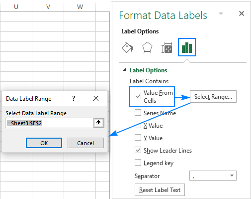
How to Use Cell Values for Excel Chart Labels Select the chart, choose the "Chart Elements" option, click the "Data Labels" arrow, and then "More Options." Uncheck the "Value" box and check the "Value From Cells" box. Select cells C2:C6 to use for the data label range and then click the "OK" button. The values from these cells are now used for the chart data labels. Pie Chart display only certain labels Trying to limit the labels on the pie chart. I understand that "#PERCENT" provides the percent labels for the pie chart. BUT I am looking to only display percent labels if they are greater than say.. 3%. Is this possible? · Ok, if you still have data to show but just not the labels, then you will have to extract the pie chart template and set up data ... How to hide zero data labels in chart in Excel? Sometimes, you may add data labels in chart for making the data value more clearly and directly in Excel. But in some cases, there are zero data labels in the chart, and you may want to hide these zero data labels. Here I will tell you a quick way to hide the zero data labels in Excel at once. Hide zero data labels in chart Solved: Show data label only to one line - Microsoft Power ... 1. Creating a separate measure for each item in your legend, like calculate (, [legendcolumn] = "legend value") 2. Remove the legend and the current measure from the line chart. 3. Add all of the measures to the line chart. 4. Then Data Labels will have the Customize Series option. View solution in original post.
Label Specific Excel Chart Axis Dates - My Online Training Hub Step 1 - Insert a regular line or scatter chart. I'm going to insert a scatter chart so I can show you another trick most people don't know*. Step 2 - Hide the line for the 'Date Label Position' series: Step 3 - Set the desired minimum and maximum dates (Scatter Charts Only) Find, label and highlight a certain data point in Excel ... Select the Data Labels box and choose where to position the label. By default, Excel shows one numeric value for the label, y value in our case. To display both x and y values, right-click the label, click Format Data Labels…, select the X Value and Y value boxes, and set the Separator of your choosing: Label the data point by name How to add data labels from different column in an Excel ... Click any data label to select all data labels, and then click the specified data label to select it only in the chart. 3. Go to the formula bar, type =, select the corresponding cell in the different column, and press the Enter key. See screenshot: 4. Repeat the above 2 - 3 steps to add data labels from the different column for other data points. Highlight a Specific Data Label in an Excel Chart ... * right click on the series, choose Change Series Chart Type from the pop up menu, and select the desired chart type. Add data labels to each line chart* (left), then format them as desired (right). * right click on the series, choose Add Data Labels from the pop up menu. Finally format the two line chart series so they use no line and no marker.
excel - How do I update the data label of a chart? - Stack Overflow
Display every "n" th data label in graphs - Microsoft ... you can use a free tool created by Rob Bovey, called the XY Chart Labeler. With this tool you can assign a range of cells to be the labels for chart series, instead of the Excel defaults. Using a formula, you can have a text show up in every nth cell and then use that range with the XY Chart Labeler to display as the series label.

How to Only Show Selected Data Points in an Excel Chart ... Download Free Sample Dashboard Files here: on how to show or hide specific data points i...
Find, label and highlight a certain data point in Excel scatter graph
How to Conditionally Show or Hide Charts - Excel Chart ... In a complicated Excel 2003 chart, which has two 4-point area chart series to highlight a background range, and an XY series with custom markers (pasted shapes) and more then 4 points, only the first four points appear with their custom markers, though the code that applies the markers does not fail, and the data labels for the marker-less ...
Creating a chart with dynamic labels - Microsoft Excel 2016
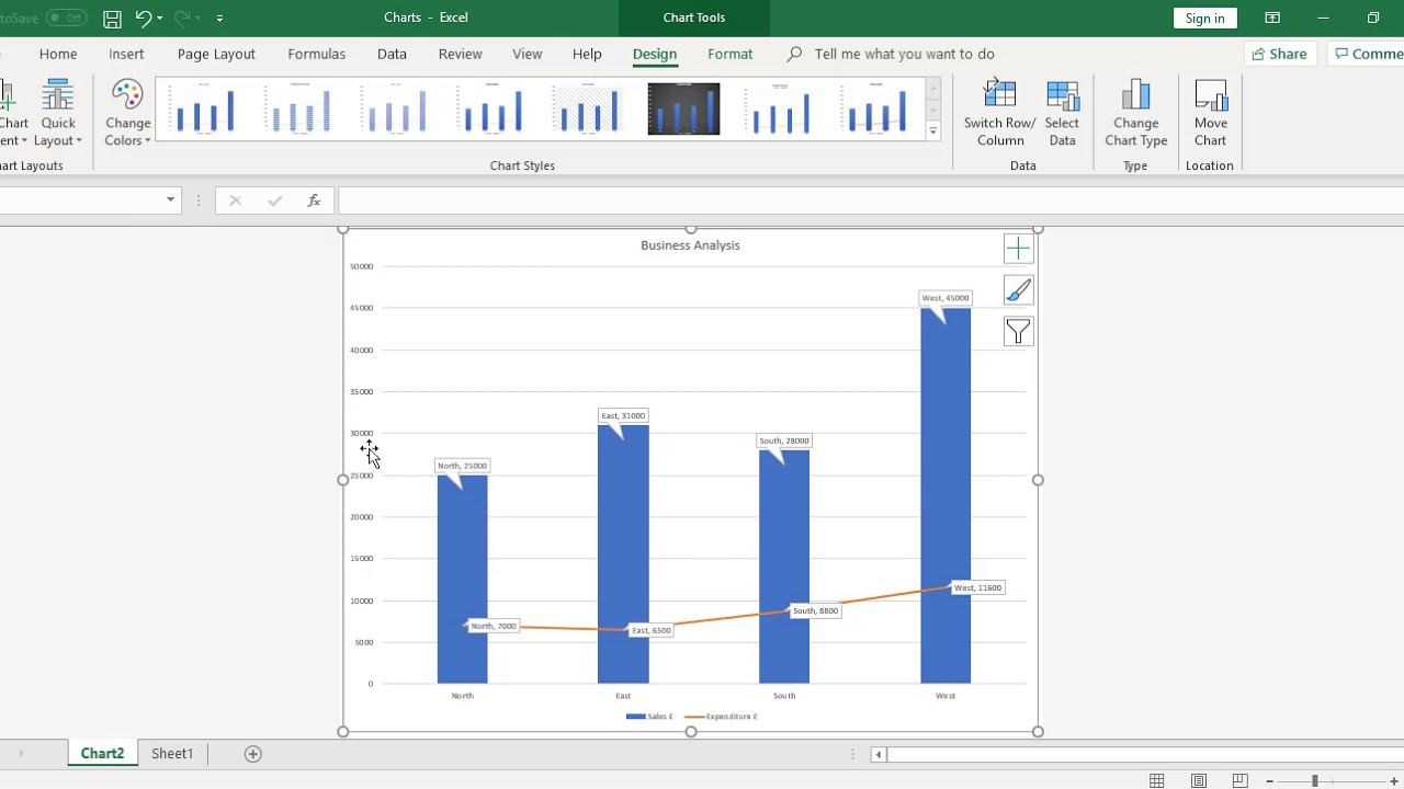
Add or remove data labels in a chart Click the data series or chart. To label one data point, after clicking the series, click that data point. In the upper right corner, next to the chart, click Add Chart Element > Data Labels. To change the location, click the arrow, and choose an option. If you want to show your data label inside a text bubble shape, click Data Callout.
Formula Friday - Using Formulas To Add Custom Data Labels To Your Excel Chart - How To Excel At ...
charts - Excel, giving data labels to only the top/bottom ... 1) Create a data set next to your original series column with only the values you want labels for (again, this can be formula driven to only select the top / bottom n values). See column D below. 2) Add this data series to the chart and show the data labels. 3) Set the line color to No Line, so that it does not appear! 4) Volia! See Below! Share

30 Label Data Points In Excel - Labels For You
Excel Chart - Do not Hide Horizontal Data Label - Stack ... 1) You can't see all your data labels on the X axis unless you format the X axis to have major interval of 1. 2) With a scatter plot, you cannot have your original labels retained on the X axis and, in your case, as your dates are recognised , they are ordered as such.
How To Add Data Labels To A Chart in Microsoft Excel - YouTube
Apply Custom Data Labels to Charted Points - Peltier Tech First, add labels to your series, then press Ctrl+1 (numeral one) to open the Format Data Labels task pane. I've shown the task pane below floating next to the chart, but it's usually docked off to the right edge of the Excel window. Click on the new checkbox for Values From Cells, and a small dialog pops up that allows you to select a ...

How to hide zero value rows in pivot table?
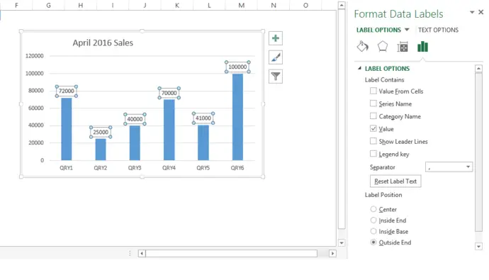
Excel tutorial: How to use data labels Generally, the easiest way to show data labels to use the chart elements menu. When you check the box, you'll see data labels appear in the chart. If you have more than one data series, you can select a series first, then turn on data labels for that series only. You can even select a single bar, and show just one data label.
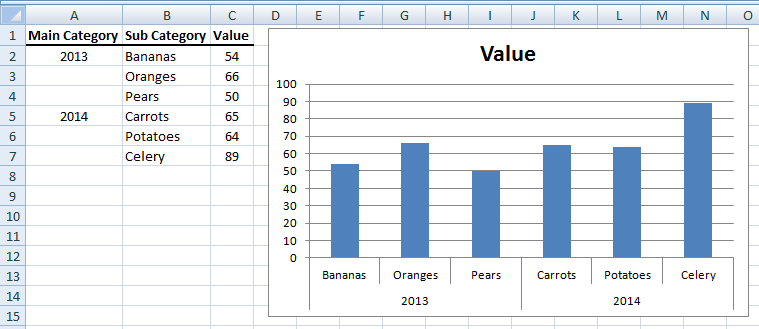
Fixing Your Excel Chart When the Multi-Level Category Label Option is Missing. - Excel Dashboard ...
Excel charts: add title, customize chart axis, legend and ... To change what is displayed on the data labels in your chart, click the Chart Elements button > Data Labels > More options… This will bring up the Format Data Labels pane on the right of your worksheet. Switch to the Label Options tab, and select the option (s) you want under Label Contains:

Only Label Specific Dates in Excel Chart Axis - Reduce ... Date axes can get cluttered when your data spans a large date range. Use this easy technique to only label specific dates.Download the Excel file here: https...

How to Add Data Labels to your Excel Chart in Excel 2013 - YouTube
Only Display Some Labels On Pie Chart - Excel Help Forum Hi All, I have a pie chart that contains over 50 categories (Yes, I know pie charts shouldn't be used for that many things) but I want to only display labels for maybe the top 5 values or any label with a value >10. This is because there are a few standout values but I want all the other values to remain in the chart as it keeps the size of the larger values in context, i just dont want this ...
Excel Formulas Tricks
Excel Chart delete individual Data Labels First select a data label, which will select all data labels in the series. You should see dark dots selecting each data label. Now select the data label to be deleted. This should remove the selection from all other labels and leave the specific data label with white selection dots. Deletion now will remove just the selected data point.
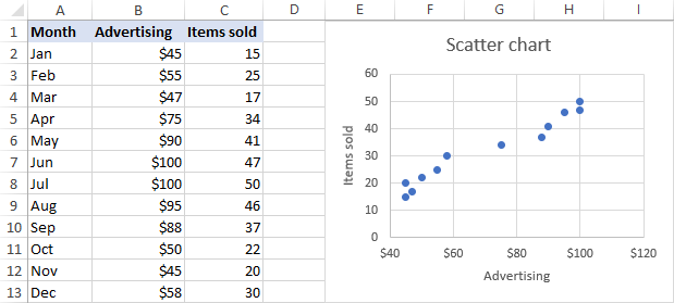
Find, label and highlight a certain data point in Excel scatter graph
Hiding certain series in an excel data table (but ... Create the chart with all 3 series (i.e. the three series and the total) as a stacked chart. Then right-click on the 'Total' series, select Chart Type and change it to a line chart. Lastly, double-click the line and format it to have no line or markers. It should then be included in the data table, but not be visible in the chart. Report abuse


How to Create a Chart in Microsoft Excel - Tech Support

Category Label disappearsExcel Chart not displaying X AxisExcel custom axis labelHow do I make ...

SSRS Charts with Data Tables (Excel Style) | Some Random Thoughts
Post a Comment for "45 excel chart only show certain data labels"