40 labels and values in excel
User-Defined Formats (Value Labels) - SAS Tutorials ... The most common way of labeling data is to simply assign each unique code its own label. Here, the format LIKERT_SEVEN assigns distinct labels to the values 1, 2, 3, 4, 5, 6, 7. How to Make a Frequency Distribution Table & Graph in Excel? By default, Excel will not display the values below 21 and above 100 as we have set Starting at value as 21 and Ending at value as 100. But you can force to display the empty bins. To display empty items, you have to right-click on any cell under Row Labels and choose Field Settings from the shortcut menu.
Series.DataLabels method (Excel) | Microsoft Docs Return value. Object. Remarks. If the series has the Show Value option turned on for the data labels, the returned collection can contain up to one label for each point. Data labels can be turned on or off for individual points in the series. If the series is on an area chart and has the Show Label option turned on for the data labels, the returned collection contains only a single label ...

Labels and values in excel
How to Create and Customize a Treemap Chart in Microsoft Excel Select the chart and go to the Chart Design tab that displays. Use the variety of tools in the ribbon to customize your treemap. For fill and line styles and colors, effects like shadow and 3-D, or exact size and proportions, you can use the Format Chart Area sidebar. Either right-click the chart and pick "Format Chart Area" or double-click ... How to Create a Histogram in Excel [Step by Step Guide] A column chart typically has text values in this axis, such as names of cities. There are no gaps between the columns of a conventional histogram. 100% of the values in a data set must be included in a histogram. A column chart could be used to compare only the top 5 products. 3. How to create a histogram in Excel with the histogram chart X Axis Labels Below Negative Values - Beat Excel! To do so, double-click on x axis labels. This will open "Format Axis" menu on left side of the screen. Make sure "Format Axis" menu is selected and if not, click on the area marked with dark green. This will open Format Axis menu. Then click on "Labels" as shown below. While in Labels menu, navigate to label position and select "Low".
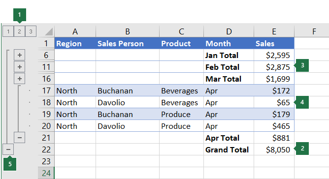
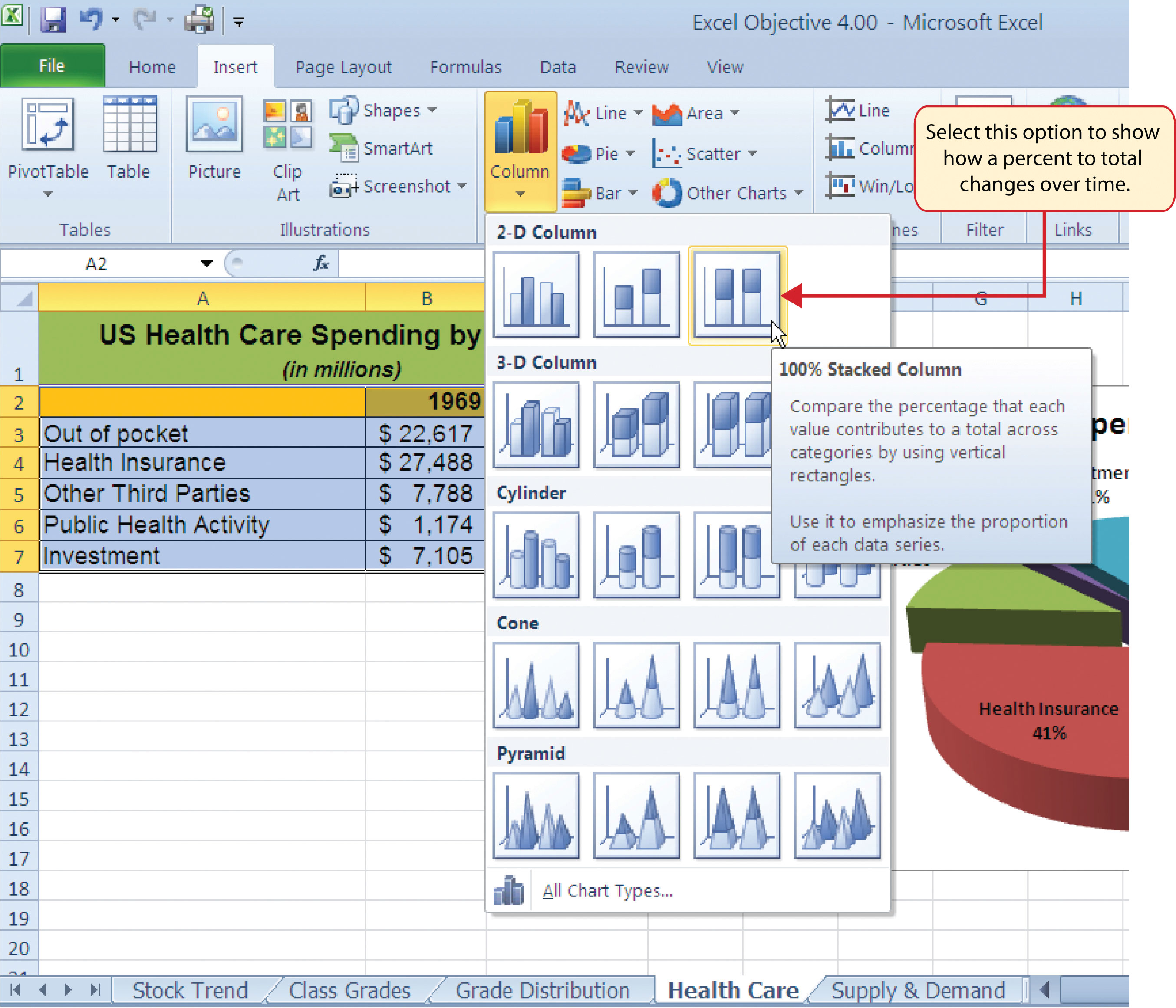
Labels and values in excel. How To Summarize Data in Excel: Top 10 Ways - ExcelChamp Calculate SUM: Click on the Autosum icon on the Home tab of Microsoft Office to activate the Sum function of Excel. Then select the data range of the column you want to summarize. Here's an example: Calculate COUNT: Click on the drop-down icon on the Autosum button on the Home tab of Microsoft Excel. How to Make a Bar Graph in Excel - Lifewire Highlight the cells you want to graph, including the labels, values and header. Open the Insert menu. In the Charts group, select the drop-down menu next to the Bar Charts icon. Select More Column Charts.; Choose Bar and select one of the six formats. Select OK to position the chart in the spreadsheet. Modify the bar graph using the tools provided. how to make a scatter plot in Excel — storytelling with data Then, we'll right-click on our chart, choose " Select Data… " from the menu that pops up, and add another data series just for our average values. Click the "+" button below the "Legend entries (Series):" window to add a new series, which you can then rename and set the range of X and Y values for in that pop-up. How to Print Labels from Excel - Lifewire Select Mailings > Write & Insert Fields > Update Labels . Once you have the Excel spreadsheet and the Word document set up, you can merge the information and print your labels. Click Finish & Merge in the Finish group on the Mailings tab. Click Edit Individual Documents to preview how your printed labels will appear. Select All > OK .
Prevent Overlapping Data Labels in Excel Charts - Peltier Tech To compile all the labels, the program builds a two-column VBA array, with series numbers in the first column and vertical position in the second. The code bubble-sorts this array by the second column. Then it loops through the series numbers in a nested loop, to compare each label with every other label. The VBA Routines How to perform VLOOKUP in Power Query without using Merge ... How to LOOKUP values in Power Query without using Merge Join in Power BI. ... Labels: Power_BI, Power_M-Query. No comments: Post a Comment. ... The 'Excel Kingdom Blog' Admin/Author believes that the information herein was Prepared by Author as well as some content written here by studying some reliable sources and posted here as is but ... How to Change the Y Axis in Excel - Alphr To change the axis label's position, go to the "Labels" section. Click the dropdown next to "Label Position," then make your selection. Changing the Display of Axes in Excel Modifying Axis Scale Labels (Microsoft Excel) In the Category list, choose Custom. In the Type box, enter a zero followed by a comma. Click OK. Only the thousands portion of the values in the axis should be displayed. You can then add another label, as desired, that indicates the values are expressed in thousands.
Format Chart Axis in Excel - Axis Options (Format Axis ... Labels are nothing but the axis values. We can change the position of axis values relative to the position of the axis line. For now, we are setting the label's position to high. Axis Options : Number Format We can change the format of axis values of the chart in excel in the same way we do for the cell entries. Excel Pivot Table tutorial - how to make and use ... To do this, in Excel 2013 and higher, go to the Insert tab > Charts group, click the arrow below the PivotChart button, and then click PivotChart & PivotTable. In Excel 2010 and 2007, click the arrow below PivotTable, and then click PivotChart. 3. Arranging the layout of your pivot table report How to Find, Highlight, and Label a Data Point in Excel ... By default, the data labels are the y-coordinates. Step 3: Right-click on any of the data labels. A drop-down appears. Click on the Format Data Labels… option. Step 4: Format Data Labels dialogue box appears. Under the Label Options, check the box Value from Cells . Step 5: Data Label Range dialogue-box appears. Pivot Table "Row Labels" Header Frustration - Microsoft ... Hi Everyone please help I can't change my headers from Row Labels in a Pivot Table. Using Excel 365
Coordinate Graph Paper Template Axis Labels » ExcelTemplate.net
How to Select Parts of Excel Pivot Table To select the Labels and Values: Select Row or Column labels, as described in the previous section. On the Excel Ribbon, click the Options tab. In the Actions group, click Select Click Labels and Values Get the Sample File You can download the zipped Pivot Table Selection sample file for this tutorial.

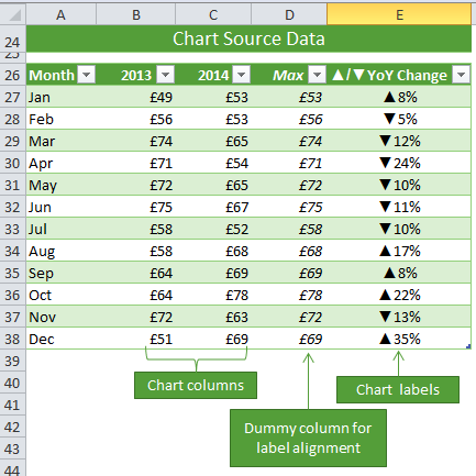
Directly Labeling Excel Charts - PolicyViz
How to Make a Scatter Plot in Excel and Present Your Data Add Labels to Scatter Plot Excel Data Points. You can label the data points in the X and Y chart in Microsoft Excel by following these steps: Click on any blank space of the chart and then select the Chart Elements (looks like a plus icon). Then select the Data Labels and click on the black arrow to open More Options. Now, click on More Options ...
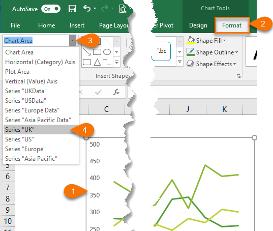
Dynamically Label Excel Chart Series Lines • My Online Training Hub
How to mail merge and print labels from Excel - Ablebits If the Use the current document option is inactive, then select Change document layout, click the Label options… link, and then specify the label information. Configure label options. Before proceeding to the next step, Word will prompt you to select Label Options such as: Printer information - specify the printer type.
How to change x axis values in Microsoft excel - YouTube
How to Add Labels to Scatterplot Points in Excel - Statology Step 3: Add Labels to Points Next, click anywhere on the chart until a green plus (+) sign appears in the top right corner. Then click Data Labels, then click More Options… In the Format Data Labels window that appears on the right of the screen, uncheck the box next to Y Value and check the box next to Value From Cells.

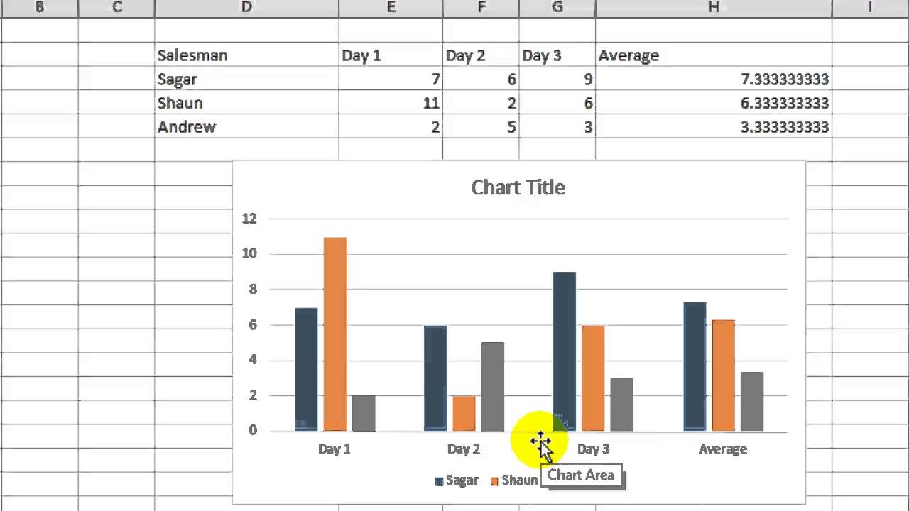
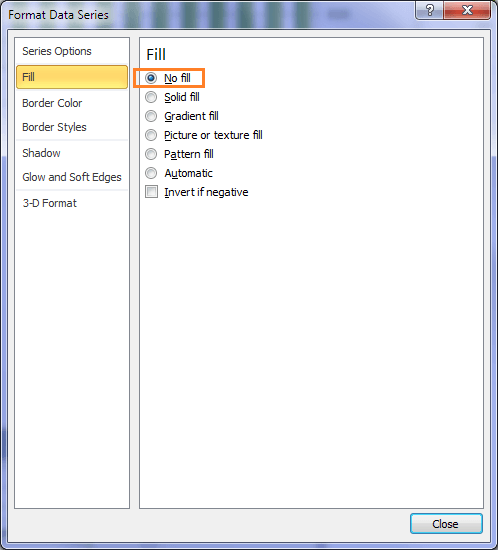
One click to add total label to stacked chart in Excel
How To Show Two Sets of Data on One Graph in Excel in 8 ... 1. Enter data in the Excel spreadsheet you want on the graph. To create a graph with data on it in Excel, the data has to be represented in the spreadsheet. For multiple variables that you want to see plotted on the same graph, entering the values into different columns is a way to ensure that the data is already in the spreadsheet.
Excel Custom Chart Labels • My Online Training Hub
5 New Charts to Visually Display Data in Excel 2019 - dummies Excel 2019 makes the process much easier with the filled map chart type. It recognizes countries, states/provinces, counties, and postal codes in data labels, and it displays the appropriate map and places the values in the appropriate areas on the map.
35 Label In Excel Definition - Labels Database 2020
How to Use Excel Pivot Table Label Filters Right-click a cell in the pivot table, and click PivotTable Options. Click the Totals & Filters tab Under Filters, add a check mark to 'Allow multiple filters per field.' Click OK Quick Way to Hide or Show Pivot Items Easily hide or show pivot table items, with the quick tip in this video. The written instructions are below the video
Download Kutools for Excel 23.00
How to Create Multi-Category Charts in Excel ... Step 1: Insert the data into the cells in Excel. Now select all the data by dragging and then go to "Insert" and select "Insert Column or Bar Chart". A pop-down menu having 2-D and 3-D bars will occur and select "vertical bar" from it. Select the cell -> Insert -> Chart Groups -> 2-D Column Bar Chart Insertion Multi-Category Chart

How to Make a Bell Curve in Excel: Example + Template
Columns and rows are labeled numerically - Office ... To change this behavior, follow these steps: Start Microsoft Excel. On the Tools menu, click Options. Click the Formulas tab. Under Working with formulas, click to clear the R1C1 reference style check box (upper-left corner), and then click OK.
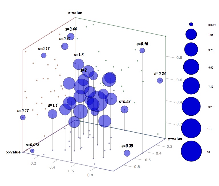
3d scatter plot for MS Excel
Custom Chart Data Labels In Excel With Formulas Follow the steps below to create the custom data labels. Select the chart label you want to change. In the formula-bar hit = (equals), select the cell reference containing your chart label's data. In this case, the first label is in cell E2. Finally, repeat for all your chart laebls.
Excel Custom Chart Labels • My Online Training Hub
X Axis Labels Below Negative Values - Beat Excel! To do so, double-click on x axis labels. This will open "Format Axis" menu on left side of the screen. Make sure "Format Axis" menu is selected and if not, click on the area marked with dark green. This will open Format Axis menu. Then click on "Labels" as shown below. While in Labels menu, navigate to label position and select "Low".
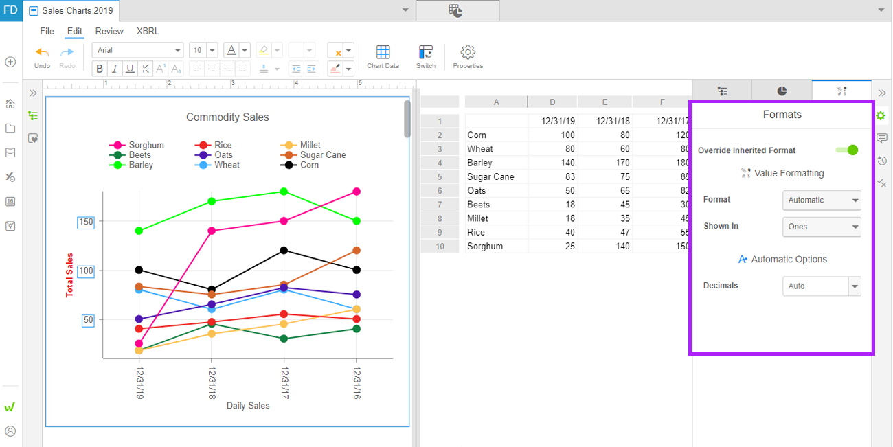
Value formats for chart labels – Workiva Support Center
How to Create a Histogram in Excel [Step by Step Guide] A column chart typically has text values in this axis, such as names of cities. There are no gaps between the columns of a conventional histogram. 100% of the values in a data set must be included in a histogram. A column chart could be used to compare only the top 5 products. 3. How to create a histogram in Excel with the histogram chart

How to create a gauge chart in Excel for great looking dashboards
How to Create and Customize a Treemap Chart in Microsoft Excel Select the chart and go to the Chart Design tab that displays. Use the variety of tools in the ribbon to customize your treemap. For fill and line styles and colors, effects like shadow and 3-D, or exact size and proportions, you can use the Format Chart Area sidebar. Either right-click the chart and pick "Format Chart Area" or double-click ...
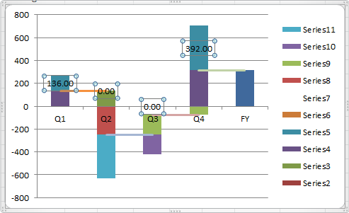
How to Create Waterfall Charts in Excel - Excel Tactics
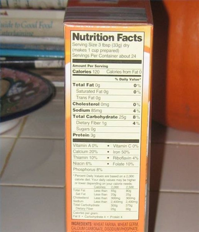
How to Make Nutrition Facts Labels | Techwalla
30 Definition Of Label In Excel - Labels Information List
Post a Comment for "40 labels and values in excel"